https://soccerda.tistory.com/131
회귀모델의 판별식 R2, RMSE
#RMSE 구하기 from sklearn.metrics import mean_squared_error def RMSE(y_test, y_predict): return np.sqrt(mean_squared_error(y_test, y_predict)) print("RMSE : ", RMSE(y_test, y_predict)) RMSE(평균 제..
soccerda.tistory.com
R2는 1에 가까울수록 RMSE는 낮을수록 좋은 수치이다.
아직 데이터가 적은 양이어서 Validation을 추가했다고 더 좋은 값이 나오는 것이 눈에 띄지 않지만, 많아질수록 Train 데이터에서 일부의 검증 세트를 분리하여 훈련하는 것이 효과적인 것을 알게 될 것이다.
#1. 데이터
import numpy as np

# 100개 데이터
x = np.array(range(1,101))
y = np.array(range(1,101))

# 6:2:2로 train validation test 세트
x_train = x[:60]
x_val = x[60:80]
x_test = x[80:]
y_train = y[:60]
y_val = y[60:80]
y_test = y[80:]

#2. 모델 구성
from keras.models import Sequential
from keras.layers import Dense
model = Sequential()

# model.add(Dense(5, input_dim = 1, activation = 'relu'))
model.add(Dense(5, input_shape = (1, ), activation ='relu'))
model.add(Dense(3))
model.add(Dense(4))
model.add(Dense(1))

# model.summary())

#3. 훈련
# model.compile(loss='mse', optimizer='adam', metrics=['accuracy'])
model.compile(loss='mse', optimizer='adam', metrics=['mse'])
model.fit(x_train, y_train, epochs=1000, batch_size=1, validation_data=(x_val, y_val))

#4. 평가 예측
mse = model.evaluate(x_test, y_test, batch_size=1)
print("mse :", mse)

y_predict = model.predict(x_test)
print(y_predict)

#RMSE 구하기
from sklearn.metrics import mean_squared_error
def RMSE(y_test, y_predict):
   return np.sqrt(mean_squared_error(y_test, y_predict))
print("RMSE :", RMSE(y_test, y_predict))

# R2 구하기
from sklearn.metrics import r2_score
f2_y_predict = r2_score(y_test, y_predict)
print("R2 :", r2_y_predict)
mse, rmse 모두 아주 낮은 수치가 나오고 R 역시 1에 근접하는 아주 좋은 평가가 나온다.
하지만 이 모델에는 약간의 문제점이 있다.
x_test값으로 predict 한 것이다. 가급적 test 한 값보다는 새로운 데이터로 예측하는 것이 좋다.
x_predict를 새로 입력하여 예측하자. x_predict는 x의 범위 바깥쪽의 새로운 데이터로 하겠다.
101에서 110까지의 값을 x로 주고예측
#1. 데이터
import numpy as np

# 100개 데이터
x = np.array(range(1,101))
y = np.array(range(1,101))
#print(x)

# 6:2:2로 train validation test 세트
x_train = x[:60]
x_val = x[60:80]
x_test = x[80:]
y_train = y[:60]
y_val = y[60:80]
y_test = y[80:]
# x_predict 추가
x_predict = np.array(range(101,111))

#2. 모델 구성
from keras.models import Sequential
from keras.layers import Dense
model = Sequential()

# model.add(Dense(5, input_dim = 1, activation = 'relu'))
model.add(Dense(5, input_shape = (1, ), activation ='relu'))
model.add(Dense(3))
model.add(Dense(4))
model.add(Dense(1))

# model.summary())

#3. 훈련
# model.compile(loss='mse', optimizer='adam', metrics=['accuracy'])
model.compile(loss='mse', optimizer='adam', metrics=['mse'])
# model.fit(x, y, epochs=100, batch_size=3)
model.fit(x_train, y_train, epochs=300, batch_size=1, validation_data=(x_val, y_val))

#4. 평가 예측
mse = model.evaluate(x_test, y_test, batch_size=1)
print("mse :", mse)

# y_predict = model.predict(t_test)
y_predict = model.predict(x_predict)
print(y_predict)
위에서는 데이터를 직접 분할하여 사용했는데 사이킷 런에서는 제공하는 train_test_split 함수를 할 수 있다.
from sklearn.model_selection import train_test_split
x_train, x_test, y_train, y_test = train_test_split(x, y, random_state=66, test_size=0.4, shuffle=False)
x, y에 데이터의 x값과 y값을 넣는다. test_size=0.4는 test_size가 40%라는 의미이다. 마찬가지로 train_size 0.6이라고 할 수도 있다. 그러면 train이 60% test가 40%로 동일한 결과가 된다. train_size와 test_size둘중 편한걸 사용하면 되고 둘을 동시에 사용할 경우 train_size를 우선으로 잘리게 된다.
그리고 shuffle은 데이터를 섞는 옵션이다. True이면 섞고 False는 섞지 않는다. 이때 중요한 것은 x와 y의 쌍까지 섞지는 않는다.
예를 들어 x=(1,2,3), y=(4,5,6)일 때 shuffle해서 x =(2,3,1), y=(4,6,5) 로는 바뀌지 않는다. 1과 4, 2와 5, 3과 6 쌍 자체가 바뀌지 않는다.
결국 x=(2,3,1) 이면 y=(5,6,4)가 된다.
적용하면
#1. 데이터
import numpy as np

# 100개 데이터
x = np.array(range(1,101))
y = np.array(range(1,101))

# 6:2:2로 train validation test 세트
#x_train = x[:60]
#x_val = x[60:80]
#x_test = x[80:]
#y_train = y[:60]
#y_val = y[60:80]
#y_test = y[80:]

from sklearn.model_selection import train_test_split
x_train, x_test, y_train, y_test = train_test_split(
   x, y, random_state=66, test_size=0.4, shuffle=False
)
validation을 만들기 위해 한번더 train_test_split를 적용시키자
x_val, x_test, y_val, y_test = train_test_split(
   x_test, y_test, random_state=66, test_size=0.5
)
Test 데이터의 50%를 validation에 배분하여 전체적으로 train:val:test의 비율이 6:2:2가 된다.
전체 소스
#1. 데이터
import numpy as np
# 100개 데이터
x = np.array(range(1,101))
y = np.array(range(1,101))
# 6:2:2로 train validation test 세트
#x_train = x[:60]
#x_val = x[60:80]
#x_test = x[80:]
#y_train = y[:60]
#y_val = y[60:80]
#y_test = y[80:]
from sklearn.model_selection import train_test_split
x_train, x_test, y_train, y_test = train_test_split(
x, y, random_state=66, test_size=0.4, shuffle=False
)
x_val, x_test, y_val, y_test = train_test_split(
x_test, y_test, random_state=66, test_size=0.5, shuffle=False
)
#2. 모델 구성
from keras.models import Sequential
from keras.layers import Dense
model = Sequential()
# model.add(Dense(5, input_dim = 1, activation ='relu'))
model.add(Dense(5, input_shape = (1, ), activation ='relu'))
model.add(Dense(3))
model.add(Dense(4))
model.add(Dense(1))
#3. 훈련
model.compile(loss='mse', optimizer='adam', metrics=['mse'])
model.fit(x_train, y_train, epochs=300, batch_size=1, validation_data=(x_val, y_val))
#4. 평가 예측
mse = model.evaluate(x_test, y_test, batch_size=1)
print("mse : ", mse)
y_predict = model.predict(x_test)
print(y_predict)
#RMSE 구하기
from sklearn.metrics import mean_squared_error
def RMSE(y_test, y_predict):
return np.sqrt(mean_squared_error(y_test, y_predict))
print("RMSE : ", RMSE(y_test, y_predict))
# R2 구하기
from sklearn.metrics import r2_score
r2_y_predict = r2_score(y_test, y_predict)
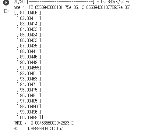
print("R2 : ", r2_y_predict)
mse, RMSE는 낮고 R2는 0.9999로 모두 매우 좋은 결과 값이다.
'AI > DeepLearning' 카테고리의 다른 글
| 회귀 모델 정리 - 순차모델 (0) | 2020.07.07 |
|---|---|
| 회귀 모델 5 - 함수형 모델 (1:1, 다:다, 다:1, 1:다) (0) | 2020.07.01 |
| 회귀 모델 3 훈련세트, 검증세트, 테스트세트 분리 (0) | 2020.06.26 |
| 회귀모델의 판별식 R2, RMSE (0) | 2020.06.23 |
| 회귀 모델 2 101~110 예측하기 (0) | 2020.06.23 |